Digital Filters

---

In the broadest sense, a filter is any function that takes input samples, modifies them in some way, and produces output samples. However, in music applications, we usually think of filters as those functions that alter the spectrum of the sound by amplifying or attenuating selected frequencies.

The mathematics involved in understanding and designing filters is complex and a detailed explanation is beyond the goals of this website.  For those who need a more detalied explanation, or need to design filters, that information can be found in books on digital signal processing (see the links in the right sidebar). For the purposes of understanding how to create the program, we will take a simpler, more intuitive approach to understanding digital filters.

If we add a sine wave to itself the resulting signal will be of the same phase and frequency but doubled in amplitude as shown below.

 Sum of sin waves

If we then shift the input signal by 180° before adding, the input values cancel and produce no output.

 Sum of sin waves, 180° phase shift

As the phase difference of the two waveforms increases from 0 to 180°, the amplitude of the sum decreases from 2 to 0. For example, at 90° phase difference the amplitude of the output signal is 1.4142. Notice that the phase of the output signal is shifted as well.

Sum of sin waves, 90° phase shift

For a digitized signal, we can sum waveforms by adding samples together and a phase shift can be created by delaying the samples one or more sample times. If we store each sample in a buffer and then later add that sample back to the current sample, we have summed the signal with a phase-shifted version of itself. We can represent the sum of the signal and delayed sample with a diagram as shown in the following figure. The delayed sample is represented by the box labeled z^-1. An amplitude multiplier is shown by the triangles.

Filter Diagram

When a delayed sample is summed with the current sample, the amount of phase shift is dependent on the sample rate, amplitude and frequency of the signal. For example, at a sample rate of 10kHz, one sample delay is equal to the sample time of 0.0001 seconds. For a signal of 100Hz, the time of one period is 0.01 seconds and a one sample delay represents 1/100 of the period, or 3.6° of phase difference. A signal at 1000Hz has a period of 0.001 seconds and a one sample time delay would be 1/10 of the period, or 36°. Since a larger phase difference results in a lower amplitude, a higher frequency signal is attenuated more than a lower frequency signal. The effect is that of a low-pass filter.

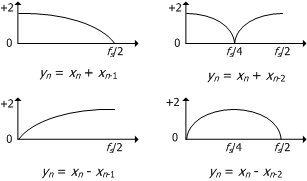
The low-pass filter created by summing a one sample delay will have an amplitude of 2 at "zero" frequency and amplitude of 0 at f_s/2. In other words, at f_s/2 the period of the waveform is only 2 samples long and a one sample delay represents half the period, or 180° phase shift. The peak amplitude for any frequency in between varies from 2 to 0.

With a two sample delay, the amplitude will be 0 at f_s/4 and will then increase back to 2 at f_s/2. Thus, a two sample delay produces a "notch" filter with a center frequency at 1/4 the sample rate.

If we subtract the delayed sample rather than add, the amplitude will be 0 when the phase difference is 0° and increase to a maximum of 2 at 180° phase difference. The effect is that of a high-pass filter. With a two sample delay, the result is a band-pass filter with the center frequency at 1/4 the sample rate. The various filtering effects are shown below.

Frequency Response of Simple Filters

As additional delay times are added, the filter output develops additional notches or bumps and the resulting frequency response looks like a comb. Thus, a filter of this type is usually referred to as a comb filter.

We can multiply the current and delayed samples by a value less than one in order to further affect the output amplitude. As the amplitude of the delayed sample is reduced, the filtering effect is reduced as well and the curve becomes flatter.

Implemented as a computer program, a digital filter is simply a sum of the input and delayed sample(s) multiplied by their respective coefficients.

output = (input * ampIn) + (delay * ampDel);
delay = input;

We can create a very "cheap" low pass filter by taking the average of the current sample and the previous sample, (a=b= 0.5). This filter has a frequency response from 0Hz to f_s/2 with a very slow roll-off. As an general audio filter it has limited usefulness. However, there are a few situations where it is quite useful, despite its simplicity.

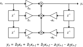
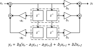
More complex filters can be constructed by combining the different types of filters shown above. By varying the number of delays, and the coefficients for the delays, a variety of filters can be created. This leads ultimately to the basic filter form known as a bi-quad filter. The bi-quad filter combines one and two sample feedforward delays with one and two sample feedback delays.

The diagram on the left shows the filter in Direct Form I, with the feed-forward delays on the left and the feedback delays on the right. Since the filter sections are commuative, we can rearrange them into the form shown on the right, Direct Form II. In Direct Form II, the delay buffers can be combined so that there are only two buffers that are shared.

We can easily convert either form into a computer program as follows. The difference in terms of performance is minimal. There are some differences in how well the two forms handle overflow and round-off errors (See: The Four Direct Forms at J. Smith's web site.)

// Direct Form I

 out = (ampIn0 * in) + (ampIn1 * dlyIn1) + (ampIn2 * dlyIn2)
      - (ampOut1 * dlyOut1) - (ampOut2 * dlyOut2);
dlyOut2 = dlyOut1;
dlyOut1 = out;
dlyIn2 = dlyIn1;
dlyIn1 = in;

// Direct Form II
tmp = in - (ampOut1 * dlyBuf1) - (ampOut2 * dlyBuf2);

out = (ampIn0 * tmp) + (ampIn1 * dlyBuf1) + (ampIn2 * dlyBuf2);

dlyBuf2 = dlyBuf1;

dlyBuf1 = tmp;

To create a filter with a specific cutoff frequency and pass-band, it is necessary to calculate the appropriate coefficients for each delay. This is the complex part of filter design. Fortunately, there are a variety of programs available that will calculate the coefficients given the type of filter, cutoff frequency, pass-band, gain, etc. In those situations where the desired filter has a fixed frequency response, we can use a filter design program and then enter the values into the synthesizer program.

For variable filtering, such as that used in subtractive synthesis, we need to calculate the coefficients dynamically so that the center frequency of the filter can be changed while the synthesizer is running. This limits using filter design programs since they typically calculate the coefficients for one frequency only. If we needed to, we could pre-calculate the coefficients for a variety of frequencies and store them in a table. However, that would limit the cutoff frequencies available and is not necessary since the calculations can be made as needed.

A good filter type for audio is the Butterworth filter. This type of filter has a flat pass-band and can easily be adapted to low-pass, high-pass and band-pass operation. A second order filter will produce 12db/oct response and is good enough for most applications while requiring a minimum of calculations. It would take several pages to show the derivation of the calculations of coefficients, and that information is already available elsewhere for those who need it. For the purpose of implementing the filter, we only need the coefficients for the filters we will use.

sqr2 = 1.414213562;

if (lowpass) {

   c = 1 / tan((PI / sampleRate) * cutoffFreq);

   c2 = c * c;

   csqr2 = sqr2 * c;

   d = (c2 + csqr2 + 1);

   ampIn0 = 1 / d;

   ampIn1 = ampIn0 + ampIn0;

   ampIn2 = ampIn0;

   ampOut1 = (2 * (1 - c2)) / d;

   ampOut2 = (c2 – csqr2 + 1) / d;

} else if (highpass) {

   c = tan((PI / sampleRate) * cutoffFreq);

   c2 = c * c;

   csqr2 = sqr2 * c;

   d = (c2 + csqr2 + 1);

   ampIn0 = 1 / d;

   ampIn1 = -(ampIn0 + ampIn0)

   ampIn2 = ampIn0;

   ampOut1 = (2 * (c2 – 1)) / d;

   ampOut2 = (1 - csqr2 + c2) / d;

} else if (bandpass) {

   c = 1 / tan((PI / sampleRate) * cutoffFreq);

   d = 1 + c;

   ampIn0 = 1 / d;

   ampIn1 = 0;

   ampIn2 = -ampIn0;

   ampOut1 = (-c*2*cos(twoPI*cutoffFreq/sr)) / d;

   ampOut2 = (c – 1) / d;

}

out = (ampIn0 * in)

    + (ampIn1 * dlyIn1)

    + (ampIn2 * dlyIn2)

–    (ampOut1 * dlyOut1)

–    (ampOut2 * dlyOut2);

dlyOut2 = dlyOut1;

dlyOut1 = out;

dlyIn2 = dlyIn1;

dlyIn1 = in;

return out * gain;